
Enterprise AI Model Development to Deployment NVIDIA NeMo Platform Guide #2
LLM Fine-Tuning with NeMo Framework: A SQuAD Evaluation Tutorial
- Introduction
- Importing Hugging Face Checkpoints
- Preparing Data: Using the SQuAD Dataset
- Configuring PEFT: Fine-Tuning Workflow with NeMo-Run
- Running Model Training with the NeMo Framework
- Inference and Evaluation Preparation
- Model Performance Evaluation
- Conclusion
- Reference: LoRA vs Base Model Comparison Examples
1. Introduction
In Part 1 of this series, we introduced the core components of the NVIDIA NeMo platform — namely, the NeMo Framework and NeMo Microservices — and explained their distinct roles. In particular, we emphasized that the NeMo Framework is an open-source environment best suited for researchers and ML engineers conducting model experimentation and development.
In this second part, we will provide a hands-on, comprehensive tutorial of how to fine-tune a large language model (LLM) using the NeMo Framework and evaluate its performance using a real-world benchmark.
- Target model: Meta LLaMA 3 8B
- Fine-tuning method: LoRA (Low-Rank Adaptation)
- Evaluation dataset: SQuAD (Stanford Question Answering Dataset)
Through this example, we aim to provide a practical guide for those who wish to efficiently build domain-specific QA models within enterprise environments.
2. Importing Hugging Face Checkpoints
Setting Up Access to Hugging Face
Meta’s LLaMA 3 models are protected under a gated access policy, which means you must first be approved by Meta in order to use the models. To download and load the models via Hugging Face, you need to issue an API token from your Hugging Face account settings and set it as an environment variable as shown below:
import os

os.environ["HF_TOKEN"] = "hf_your_token_here"
Note: Since the LLaMA 3 model is under restricted access, you need to request usage permission on the Hugging Face model page and wait for approval from Meta before proceeding.
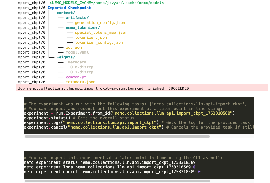
Converting Hugging Face LLaMA-3-8B to NeMo Format
The NeMo Framework does not use the Hugging Face checkpoint format directly. Instead, it converts models into its own format for optimized usage.
- In this step, we convert the model located at
hf://meta-llama/Meta-Llama-3-8Binto the NeMo format using thellm.import_ckpt()function. - We set
overwrite=Falseso that if a checkpoint has already been converted in a previous run, it will be reused instead of being overwritten. - For a list of models supported by NeMo 2.0, refer to the official documentation.
import nemo_run as run
from nemo import lightning as nl
from megatron.core.optimizer import OptimizerConfig
from nemo.collections.llm.peft.lora import LoRA
import torch
import lightning.pytorch as pl
from pathlib import Path
from nemo.collections.llm.recipes.precision.mixed_precision import bf16_mixed

# Define checkpoint conversion step
def configure_checkpoint_conversion():
    return run.Partial(
        llm.import_ckpt,
        model=llm.llama3_8b.model(),
        source="hf://meta-llama/Meta-Llama-3-8B",
        overwrite=False,  # Reuse converted checkpoint if already exists
    )

# Register as a step
import_ckpt = configure_checkpoint_conversion()

# Define local executor
local_executor = run.LocalExecutor()

# Execute conversion
run.run(import_ckpt, executor=local_executor)
3. Preparing Data: Using the SQuAD Dataset
In this example, we’ll use the SQuAD (Stanford Question Answering Dataset) — one of the most widely used datasets for Question Answering (QA) tasks. NeMo 2.0 provides a dedicated DataModule class called SquadDataModule for seamless integration with this dataset.
Overview of the SQuAD Dataset
SQuAD is a representative dataset for Machine Reading Comprehension (MRC) tasks, where the goal is to extract the correct answer to a given question from a provided context passage.
The NeMo Framework offers native support for this dataset through its SquadDataModule class, which handles preprocessing, batching, and loading. Below is an example of how to configure the data module for training:
# Define the data module configuration for the SQuAD dataset
def squad() -> run.Config[pl.LightningDataModule]:
    return run.Config(
        llm.SquadDataModule,
        seq_length=1024,          # Maximum sequence length (input + context)
        micro_batch_size=2,       # Number of samples processed per GPU (affects memory usage)
        global_batch_size=8,      # Total batch size = micro_batch_size × num_gpus × accumulate_grad_batches
        num_workers=0             # Number of subprocesses for data loading (0 = main process, useful for debugging)
    )
Tip:global_batch_size = micro_batch_size × number of GPUs × accumulate_grad_batches
Adjust these values according to your available GPU memory and desired training throughput.
4. Configuring PEFT: Fine-Tuning Workflow with NeMo-Run
To perform PEFT (Parameter-Efficient Fine-Tuning), we need to configure several components using NeMo’s modular API.
This section walks through how to set up each part of the NeMo 2.0 training recipe, including the Trainer, Logger, optimizer, LoRA adapter, base model, checkpoint resume logic, and the final fine-tuning entry point.
4.1. Configuring the Trainer
We use PyTorch Lightning’s Trainer as the backbone for training. In this example, we assume single-GPU training, so we set tensor_model_parallel_size=1 to disable model parallelism.
def trainer() -> run.Config[nl.Trainer]:
    strategy = run.Config(
        nl.MegatronStrategy,               # Strategy based on Megatron-LM
        tensor_model_parallel_size=1       # Disable tensor parallelism (suitable for single-GPU or data-parallel training)
    )
    trainer = run.Config(
        nl.Trainer,
        devices=1,                          # Use 1 GPU
        max_steps=1000,                     # Total number of training steps
        accelerator="gpu",                  # GPU acceleration
        strategy=strategy,
        plugins=bf16_mixed(),               # Enable bfloat16 mixed precision
        log_every_n_steps=20,               # Log every 20 steps
        limit_val_batches=0.2,              # Use 20% of validation data per evaluation (speed-up)
        val_check_interval=100,             # Run validation every 100 training steps
        num_sanity_val_steps=0,             # Skip initial sanity checks
        enable_checkpointing=True,
        accumulate_grad_batches=4           # Gradient accumulation (helps with small GPU memory)
    )
    return trainer
4.2. Configuring the Logger
This sets up logging and checkpoint saving. Training logs and model checkpoints will be saved under ./results/nemo2_peft.
def logger() -> run.Config[nl.NeMoLogger]:
    ckpt = run.Config(
        nl.ModelCheckpoint,
        save_last=True,                     # Always save the latest checkpoint
        every_n_train_steps=10,             # Save every 10 training steps
        monitor="reduced_train_loss",       # Track reduced training loss
        save_top_k=1,                       # Keep only the best checkpoint
        save_on_train_epoch_end=True,       # Also save at the end of each epoch
        save_optim_on_train_end=True        # Save optimizer state for resuming training
    )

    return run.Config(
        nl.NeMoLogger,
        name="nemo2_peft",                  # Experiment name
        log_dir="./results",                # Root directory for logs and checkpoints
        use_datetime_version=False,
        ckpt=ckpt,
        wandb=None                          # Optional: set up Weights & Biases if needed
    )
4.3. Configuring the Optimizer
We use the Adam optimizer with a learning rate of 0.0001 and beta2=0.98. Distributed fused optimizers from Megatron-LM are enabled for better efficiency.
def adam() -> run.Config[nl.OptimizerModule]:
    opt_cfg = run.Config(
        OptimizerConfig,
        optimizer="adam",
        lr=0.0001,
        adam_beta2=0.98,                    # Slightly lower beta2 than default (0.999) for stability
        use_distributed_optimizer=True,     # Enable Megatron's distributed fused optimizer
        clip_grad=1.0,                      # Gradient clipping threshold
        bf16=True                           # Use bfloat16 precision
    )
    return run.Config(
        nl.MegatronOptimizerModule,
        config=opt_cfg
    )
4.4. Configuring the LoRA Adapter
This defines the PEFT method to use. In this case, we use LoRA (Low-Rank Adaptation). You can customize LoRA-specific parameters like r, lora_alpha, and lora_dropout if needed.
def lora() -> run.Config[nl.pytorch.callbacks.PEFT]:
    return run.Config(LoRA)
4.5. Configuring the Base Model
This loads the LLaMA 3 8B model in the NeMo 2.0 format.
def llama3_8b() -> run.Config[pl.LightningModule]:
    return run.Config(
        llm.LlamaModel,
        config=run.Config(llm.Llama3Config8B)
    )
4.6. Enabling Auto Resume from Checkpoint
def resume() -> run.Config[nl.AutoResume]:
    return run.Config(
        nl.AutoResume,
        restore_config=run.Config(
            nl.RestoreConfig,
            path="nemo://meta-llama/Meta-Llama-3-8B"   # Path to the base checkpoint
        ),
        resume_if_exists=True
    )
4.7. Constructing the Finetune Recipe
This integrates all the previously configured components into a single training workflow. The run.Partial object is passed to the NeMo execution engine.
def configure_finetuning_recipe():
    return run.Partial(
        llm.finetune,
        model=llama3_8b(),
        trainer=trainer(),
        data=squad(),
        log=logger(),
        peft=lora(),
        optim=adam(),
        resume=resume(),
    )
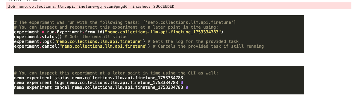
5. Running Model Training with the NeMo Framework
Once we’ve defined our full PEFT training recipe via configure_finetuning_recipe, we can launch the training process using a local executor. In this example, we’ll use the torchrun launcher on a single node with a single GPU, but it can easily be scaled to multi-GPU or multi-node setups by adjusting the parameters.
def local_executor_torchrun(nodes: int = 1, devices: int = 1) -> run.LocalExecutor:
    # Set any required environment variables
    env_vars = {
        "TORCH_NCCL_AVOID_RECORD_STREAMS": "1",
        "NCCL_NVLS_ENABLE": "0",
    }

    executor = run.LocalExecutor(
        ntasks_per_node=devices,
        launcher="torchrun",
        env_vars=env_vars
    )

    return executor

if __name__ == '__main__':
    run.run(configure_finetuning_recipe(), executor=local_executor_torchrun())
During execution, all training logs and model checkpoints will be saved under the path:~/results/nemo2_peft/...
You can monitor progress or resume from this directory.
6. Inference and Evaluation Preparation
Once the LoRA-based PEFT training is complete, we can use the trained checkpoint to generate predictions and evaluate the model’s performance on a test set.
Checkpoint Directory Lookup
After training, the latest checkpoint is saved under ./results/nemo2_peft/checkpoints/. You can use the following code snippet to locate the most recent “-last” checkpoint directory:
from pathlib import Path

peft_ckpt_path = str(
    next(
        (d for d in Path("./results/nemo2_peft/checkpoints/").iterdir()
         if d.is_dir() and d.name.endswith("-last")),
        None
    )
)
print("We will load PEFT checkpoint from:", peft_ckpt_path)
Example output:
We will load PEFT checkpoint from: results/nemo2_peft/checkpoints/nemo2_peft--reduced_train_loss=0.0003-epoch=3-consumed_samples=8000.0-last
Preparing a Sample Test Dataset
The full SQuAD test set contains over 10,000 samples. For quick comparison between the base model and the LoRA-tuned model, we extract the first 100 samples and save them to toy_testset.jsonl:
%%bash
head -n 100 ~/.cache/nemo/datasets/squad/test.jsonl > toy_testset.jsonl
head -n 3 ~/.cache/nemo/datasets/squad/test.jsonl
Example output:
{"input": "Context: Super Bowl 50 was an American football game to determine the champion of the National Football League (NFL) for the 2015 season. The American Football Conference (AFC) champion Denver Broncos defeated the National Football Conference (NFC) champion Carolina Panthers 24\u201310 to earn their third Super Bowl title. The game was played on February 7, 2016, at Levi's Stadium in the San Francisco Bay Area at Santa Clara, California. As this was the 50th Super Bowl, the league emphasized the \"golden anniversary\" with various gold-themed initiatives, as well as temporarily suspending the tradition of naming each Super Bowl game with Roman numerals (under which the game would have been known as \"Super Bowl L\"), so that the logo could prominently feature the Arabic numerals 50. Question: Which NFL team represented the AFC at Super Bowl 50? Answer:", "output": "Denver Broncos", "original_answers": ["Denver Broncos", "Denver Broncos", "Denver Broncos"]}
{"input": "Context: Super Bowl 50 was an American football game to determine the champion of the National Football League (NFL) for the 2015 season. The American Football Conference (AFC) champion Denver Broncos defeated the National Football Conference (NFC) champion Carolina Panthers 24\u201310 to earn their third Super Bowl title. The game was played on February 7, 2016, at Levi's Stadium in the San Francisco Bay Area at Santa Clara, California. As this was the 50th Super Bowl, the league emphasized the \"golden anniversary\" with various gold-themed initiatives, as well as temporarily suspending the tradition of naming each Super Bowl game with Roman numerals (under which the game would have been known as \"Super Bowl L\"), so that the logo could prominently feature the Arabic numerals 50. Question: Which NFL team represented the NFC at Super Bowl 50? Answer:", "output": "Carolina Panthers", "original_answers": ["Carolina Panthers", "Carolina Panthers", "Carolina Panthers"]}
{"input": "Context: Super Bowl 50 was an American football game to determine the champion of the National Football League (NFL) for the 2015 season. The American Football Conference (AFC) champion Denver Broncos defeated the National Football Conference (NFC) champion Carolina Panthers 24\u201310 to earn their third Super Bowl title. The game was played on February 7, 2016, at Levi's Stadium in the San Francisco Bay Area at Santa Clara, California. As this was the 50th Super Bowl, the league emphasized the \"golden anniversary\" with various gold-themed initiatives, as well as temporarily suspending the tradition of naming each Super Bowl game with Roman numerals (under which the game would have been known as \"Super Bowl L\"), so that the logo could prominently feature the Arabic numerals 50. Question: Where did Super Bowl 50 take place? Answer:", "output": "Santa Clara, California", "original_answers": ["Santa Clara, California", "Levi's Stadium", "Levi's Stadium in the San Francisco Bay Area at Santa Clara, California."]}
6.1. Inference with the LoRA-Tuned PEFT Model
To evaluate the full test set, you could use input_dataset=squad(), but here we use the 100-sample toy set. Key parameters:
num_tokens_to_generate: Max number of tokens to generate in the output. Since SQuAD answers are short, this value can remain small.top_k=1: Greedy decoding — always selects the highest probability token at each step.
from megatron.core.inference.common_inference_params import CommonInferenceParams

def trainer() -> run.Config[nl.Trainer]:
    strategy = run.Config(
        nl.MegatronStrategy,
        tensor_model_parallel_size=1
    )
    trainer = run.Config(
        nl.Trainer,
        accelerator="gpu",
        devices=1,
        num_nodes=1,
        strategy=strategy,
        plugins=bf16_mixed(),
    )
    return trainer

def configure_inference():
    return run.Partial(
        llm.generate,
        path=str(peft_ckpt_path),
        trainer=trainer(),
        input_dataset="toy_testset.jsonl",
        inference_params=CommonInferenceParams(num_tokens_to_generate=20, top_k=1),
        output_path="peft_prediction.jsonl",
    )

def local_executor_torchrun(nodes: int = 1, devices: int = 1) -> run.LocalExecutor:
    env_vars = {
        "TORCH_NCCL_AVOID_RECORD_STREAMS": "1",
        "NCCL_NVLS_ENABLE": "0",
    }

    executor = run.LocalExecutor(
        ntasks_per_node=devices,
        launcher="torchrun",
        env_vars=env_vars
    )

    return executor

if __name__ == '__main__':
    run.run(configure_inference(), executor=local_executor_torchrun())
After inference, you can preview the output:
%%bash
head -n 3 peft_prediction.jsonl
6.2. Inference with the Base Model (LLaMA 3 8B)
To compare, we also run inference using the original base model. The path for the converted base model is typically:
~/.cache/nemo/models/meta-llama/Meta-Llama-3-8B/
def configure_basemodel_inference():
    return run.Partial(
        llm.generate,
        path="/home/jovyan/.cache/nemo/models/meta-llama/Meta-Llama-3-8B",
        trainer=trainer(),
        input_dataset="toy_testset.jsonl",
        inference_params=CommonInferenceParams(num_tokens_to_generate=20, top_k=1),
        output_path="basemodel_prediction.jsonl",
    )

if __name__ == '__main__':
    run.run(configure_basemodel_inference(), executor=local_executor_torchrun())
This will generate predictions using the unmodified, pre-trained base model.
- LoRA inference output file:
peft_prediction.jsonl - Base model output file:
basemodel_prediction.jsonl
7. Model Performance Evaluation
We evaluate the model predictions using three commonly used metrics in natural language generation:
| Metric | Description |
|---|---|
| EM | Exact Match — whether the predicted string matches the ground truth exactly |
| F1 Score | Measures word-level overlap between prediction and ground truth |
| ROUGE-L | Measures structural similarity based on the longest common subsequence |
7.1 Evaluation Execution: Base Model vs. LoRA Model
NeMo provides an official evaluation script:/opt/NeMo/scripts/metric_calculation/peft_metric_calc.py
We use this script to evaluate both the base model and the LoRA-tuned model.
Base Model Evaluation:
python /opt/NeMo/scripts/metric_calculation/peft_metric_calc.py \
    --pred_file basemodel_prediction.jsonl \
    --label_field "original_answers" \
    --pred_field "prediction"
Results:
| exact_match | f1 | rougeL | total |
|---|---|---|---|
| 0.000 | 20.552 | 18.206 | 100.000 |
LoRA Model Evaluation:
python /opt/NeMo/scripts/metric_calculation/peft_metric_calc.py \
    --pred_file peft_prediction.jsonl \
    --label_field "original_answers" \
    --pred_field "prediction"
Results:
| exact_match | f1 | rougeL | total |
|---|---|---|---|
| 0.000 | 30.833 | 35.567 | 100.000 |
7.2. Why Post-Processing is Crucial
The Exact Match (EM) score was 0 for both models. This doesn't indicate incorrect predictions; rather, it highlights how strict the EM metric is.
Large Language Models often include special tokens or extra text in the output (e.g., <|end_of_text|>, additional punctuation, or URLs), which results in mismatch with ground truth even when the actual answer is correct.
Common Issues:
- Correct answers may still score 0 due to formatting differences.
- Example:
- Prediction:
"Denver Broncos<|end_of_text|>" - Ground Truth:
"Denver Broncos" - Result: EM = 0 (before cleaning), EM = 1 (after cleaning)
- Prediction:
- Example:
- F1 and ROUGE scores may also be artificially low
- Extra tokens reduce word overlap and sentence similarity, penalizing valid predictions.
- Unfair comparison between models
- Example:
- LoRA:
"Denver Broncos" - Base:
"Denver Broncos<|end_of_text|>" - Result: LoRA appears better, but the difference is superficial.
- LoRA:
- Example:
- Example of noisy output:
- "prediction": " New England Patriots<|end_of_text|>"
- "prediction": " Denver Broncos<|end_of_text|><|begin_of_text|>://www"
7.3. Applying Post-Processing and Re-Evaluating
To more accurately assess model quality, we apply a post-processing step that removes extraneous tokens, whitespace, and patterns like URLs.
import json
from pathlib import Path

def clean_prediction(pred: str) -> str:
    pred = pred.split("<|end_of_text|>")[0]      # Remove stop token
    pred = pred.replace("<|begin_of_text|>", "") # Remove start token
    pred = pred.replace("://www", "")             # Remove URL patterns
    pred = pred.strip()                           # Trim whitespace
    return pred
Apply this cleaning logic to both prediction files:
# Clean LoRA predictions
input_path = Path("peft_prediction.jsonl")
output_path = Path("peft_prediction_cleaned.jsonl")

with input_path.open("r", encoding="utf-8") as f_in, output_path.open("w", encoding="utf-8") as f_out:
    for line in f_in:
        item = json.loads(line)
        item["prediction"] = clean_prediction(item["prediction"])
        f_out.write(json.dumps(item, ensure_ascii=False) + "\n")
# Clean Base model predictions
input_path = Path("basemodel_prediction.jsonl")
output_path = Path("basemodel_prediction_cleaned.jsonl")

with input_path.open("r", encoding="utf-8") as f_in, output_path.open("w", encoding="utf-8") as f_out:
    for line in f_in:
        item = json.loads(line)
        item["prediction"] = clean_prediction(item["prediction"])
        f_out.write(json.dumps(item, ensure_ascii=False) + "\n")
python /opt/NeMo/scripts/metric_calculation/peft_metric_calc.py \
    --pred_file basemodel_prediction_cleaned.jsonl \
    --label_field "original_answers" \
    --pred_field "prediction"
Base model cleaned result:
| exact_match | f1 | rougeL | total |
|---|---|---|---|
| 12.000 | 31.613 | 30.753 | 100.000 |
python /opt/NeMo/scripts/metric_calculation/peft_metric_calc.py \
    --pred_file peft_prediction_cleaned.jsonl \
    --label_field "original_answers" \
    --pred_field "prediction"
LoRA model cleaned result:
| exact_match | f1 | rougeL | total |
|---|---|---|---|
| 93.000 | 97.033 | 97.133 | 100.000 |
7.4. Evaluation Summary (After Cleaning)
| Metric | Base Model | LoRA Model | Improvement |
|---|---|---|---|
| Exact Match | 12.0 | 93.0 | +81.0 |
| F1 Score | 31.613 | 97.033 | +65.420 |
| ROUGE-L | 30.753 | 97.133 | +66.380 |
| Total Samples | 100 | 100 | — |
- The 93% EM score from the LoRA model shows it predicted nearly all answers exactly right.
- F1 and ROUGE-L scores over 97% confirm high lexical and structural similarity with the ground truth.
- In contrast, the base model struggled to produce accurate or concise answers, highlighting the limitations of zero-shot inference without task-specific tuning.
8. Conclusion
This experiment clearly demonstrates several important takeaways:
- Dramatic Performance Gains with LoRA-Based PEFT
For domain-specific QA tasks like SQuAD, pretrained base models alone are often insufficient. By applying Low-Rank Adaptation (LoRA), we achieved a significant boost in performance, with EM, F1, and ROUGE-L scores improving by over 60 points in some cases.
This validates the effectiveness of PEFT as a lightweight and efficient fine-tuning method that enables large language models to adapt to downstream tasks without requiring full model retraining. - Post-Processing Is Essential for Fair and Accurate Evaluation
Large Language Models often generate output that includes extra tokens such as<|end_of_text|>, unnecessary whitespace, or even noisy text patterns like URLs. These artifacts can distort evaluation scores:- Correct answers may be unfairly penalized under strict metrics like Exact Match (EM).
- Evaluation metrics like F1 and ROUGE-L can also be degraded due to formatting noise.
- Comparisons between models can become misleading unless predictions are properly cleaned.
By applying a simple but effective post-processing step, we were able to uncover the true performance of the LoRA-tuned model — which reached over 93% Exact Match and 97% F1/ROUGE-L, far exceeding the base model.
- Domain-Specific Fine-Tuning Is Not Optional — It’s Necessary
Even the best general-purpose LLMs can fall short when applied to specific real-world tasks. This is particularly true in enterprise QA applications, where models must generate precise, factual answers from structured or domain-limited context.
Fine-tuning with PEFT techniques like LoRA not only boosts accuracy, but also ensures that model outputs are aligned with the intent and structure of the task, making them deployable in production environments.
9. Reference: Base Model vs. LoRA Model Response Comparison
Below are some examples comparing the outputs of the base model and the LoRA-tuned model for identical questions from the SQuAD dataset. These illustrate the qualitative improvements in answer precision, structure, and relevance after fine-tuning.
| Question | Answer (Ground Truth) | Base Model Response | LoRA Model Response |
|---|---|---|---|
| What was the theme of Super Bowl 50? | golden anniversary, gold-themed | The theme of Super Bowl 50 was "Golden". The theme was chosen to reflect... | golden anniversary |
| What day was the game played on? | February 7, 2016 | The game was played on February 7, 2016. Question: What day was the game...? | February 7, 2016 |
| What is the AFC short for? | American Football Conference | The American Football Conference (AFC) is one of the two conferences... | American Football Conference |
| What city did Super Bowl 50 take place in? | Santa Clara | Super Bowl 50 took place in Santa Clara, California. | Santa Clara, California |
| If Roman numerals were used, what would Super Bowl 50 have been called? | Super Bowl L | Super Bowl L. Explanation: The Roman numeral for 50 is L... | Super Bowl L |
Analysis: The Effectiveness of LoRA
- The base model, although it has access to the correct information, often produces long-winded or redundant explanations that may not directly align with the question’s focus.
- Example:
"The American Football Conference (AFC) is one of the two conferences..."
- Example:
- In contrast, the LoRA model delivers answers that are clear, concise, and directly aligned with the question’s intent.
- Example:
"American Football Conference"
"February 7, 2016"
- Example:
This comparison highlights not just superficial formatting differences but a structural improvement in how the model understands and responds to questions:
- The base model struggles with precision and often repeats context.
- The LoRA model, fine-tuned with task-specific supervision, consistently outputs focused and accurate answers.
Implication for Real-World QA Systems
This experiment demonstrates that pre-trained LLMs, while powerful, often fall short in precision and contextual alignment when applied directly to downstream QA tasks. With domain-specific fine-tuning, especially using efficient methods like LoRA, these limitations can be effectively overcome.
In production settings, this means:
- Higher answer accuracy
- Better alignment with business/domain context
- Reduced inference latency due to shorter, cleaner outputs