DuckDB: A Modern Analytics Database Guide

Table of Contents

• 1. Introduction
  • DuckDB Architecture and Key Features
  • Data Analysis Advantages of DuckDB
• 2. Installing DuckDB
  • Installation on Windows WSL
• 3. DuckDB Usage Examples
• 4. Conclusion
  • DuckDB's Data Analysis Advantages and Limitations

---

1. Introduction

DuckDB is an embedded analytical database that aims to be the analytical version of SQLite. It enables fast analysis of large-scale data in a local environment without requiring separate server setup, and can directly query various file formats including CSV, Parquet, and JSON. This guide covers everything from DuckDB's architecture and installation methods to various SQL examples that can be applied in real-world scenarios.

DuckDB Architecture and Key Features

DuckDB is an embedded analytical database developed to be the analytical counterpart of SQLite. Optimized for OLAP (Online Analytical Processing) workloads, it features the following core architectural characteristics.

Key Architectural Features:

• Columnar Storage: Column-based data storage optimized for analytical queries, significantly improving processing speed by reading only specific columns.
• Vectorized Query Engine: Vectorized execution that processes multiple rows at once, efficiently utilizing CPU cache.
• Embedded Database: Runs directly integrated into applications without a separate server process.
• Zero-Copy Data Access: Integration with Apache Arrow allows data sharing without memory copying.

Core Strengths:

1. Easy Installation and Use: No separate server setup or management required.
2. Excellent Performance: Benchmarks show up to tens of times faster performance compared to other embedded databases.
3. Complete SQL Support: Supports complex analytical queries, window functions, CTEs, and more.
4. Diverse Data Format Support: Can directly query CSV, Parquet, JSON, and other formats.
5. Python/R Integration: Provides seamless integration with the data science ecosystem.

Data Analysis Advantages of DuckDB

Advantages:

• Fast Analysis Speed: Fast analysis of large-scale data with columnar storage and vectorized engine.
• Memory Efficiency: Automatic memory management and disk spilling enable processing of data exceeding memory.
• Easy Data Loading: Simplifies ETL processes by allowing direct file queries.
• Standard SQL Usage: Leverages existing SQL knowledge without learning new syntax.
• Local-First Philosophy: All operations possible in local environments without cloud dependencies.

Limitations:

• OLTP Unsuitable: Not suitable for applications with heavy transactional processing.
• Concurrent Write Limitations: Not suitable for environments where multiple processes write simultaneously.
• Lack of Network Features: Does not support client-server model by default.
• Index Limitations: Traditional index structures like B-Tree indexes are limited.

2. Installing DuckDB

Installation on Windows WSL

Installing DuckDB in Windows WSL (Windows Subsystem for Linux) environment is very straightforward.

Method 1: Direct CLI Binary Download

# Download latest version
wget https://github.com/duckdb/duckdb/releases/download/v1.1.3/duckdb_cli-linux-amd64.zip

# Extract
unzip duckdb_cli-linux-amd64.zip

# Grant execution permissions
chmod +x duckdb

# Run DuckDB
./duckdb

Method 2: Install as Python Package

# Install using pip
pip install duckdb

# Use in Python
python3
>>> import duckdb
>>> duckdb.sql("SELECT 42 AS answer").show()

Verify Installation:

# Check version
./duckdb --version

# Test with a simple query
./duckdb -c "SELECT 'Hello, DuckDB!' AS greeting"

3. DuckDB Usage Examples

Downloading Example Files

Download the example files used in these examples to a specific directory (here, /mnt/c/tmp).
https://github.com/duckdb-in-action/examples

Example 1: Concise JOIN Using USING

-- Listing 3.12: Join using USING clause (equivalent to ON r1.id = r2.id)
SELECT * 
FROM (VALUES (1, 'a1'), (2, 'a2'), (3, 'a3')) l(id, nameA) 
JOIN (VALUES (1, 'b1'), (2, 'b2'), (4, 'b4')) r(id, nameB) 
USING (id);

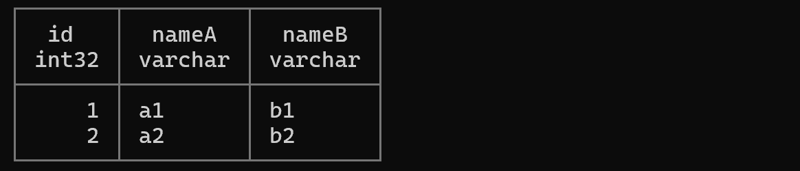
Explanation: The USING (id) syntax is a concise join method used when both tables have columns with the same name. It's equivalent to ON l.id = r.id but the id column is not duplicated in the results.

Example 2: Dynamic Column Selection with COLUMNS Expression

-- Select only columns starting with 'valid'
SELECT COLUMNS('valid.*') 
FROM "/mnt/c/tmp/ch03/prices.csv" 
LIMIT 3;

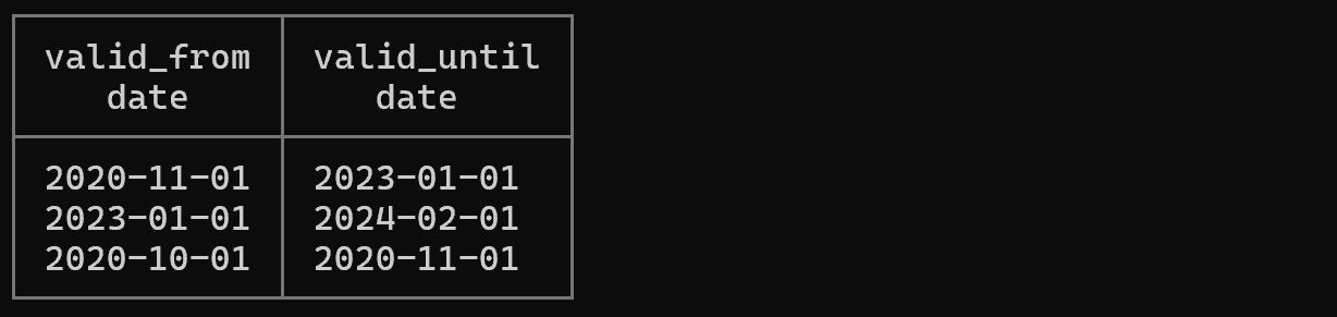
Explanation: One of DuckDB's powerful features, the COLUMNS expression allows dynamic column selection using regex patterns. This is very useful when extracting columns matching specific patterns from tables with many columns.

Example 3: SELECT * Omission Syntax

-- Query starting from FROM clause (SELECT * is implicitly applied)
FROM "/mnt/c/tmp/ch03/prices.csv" 
WHERE COLUMNS('valid.*') BETWEEN '2020-01-01' AND '2021-01-01';

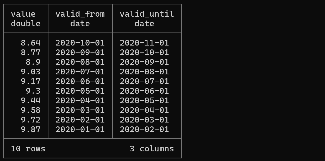
Explanation: DuckDB supports convenient syntax that allows starting queries from FROM by omitting SELECT *. This is a practical feature that reduces typing during interactive data exploration.

Example 4: Name-Based Insert Using BY NAME

-- Listing 3.19: Insert data by mapping column names
INSERT INTO systems BY NAME 
SELECT DISTINCT 
    system_id AS id, 
    system_public_name AS NAME 
FROM 'https://oedi-data-lake.s3.amazonaws.com/pvdaq/csv/systems.csv' 
ON CONFLICT DO NOTHING;

Explanation: The BY NAME keyword maps and inserts data by column name rather than position. Very useful when source and target table column orders differ, or when inserting only specific columns. Note that CSV can be read directly from URLs.

Example 5: JSON Reading with Named Parameters

# Listing 3.24: Read JSON file with date format specification
echo '{"foo": "21.9.1979"}' > 'my.json'

./duckdb -s \
  "SELECT * FROM read_json_auto(
    'my.json', 
    dateformat='%d.%M.%Y'
  )"

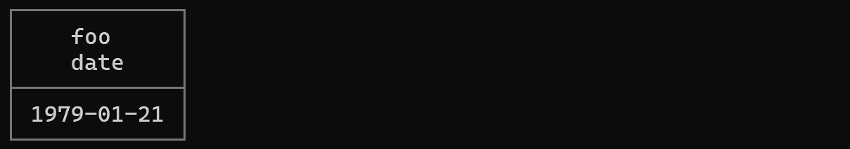
Explanation: DuckDB can automatically infer schema from JSON files and read them, with the ability to specify custom date formats using the dateformat parameter. The -s option is script mode that executes a single command and exits.

Example 6: Quick Data Exploration with SUMMARIZE

-- Automatically generate statistical summary of data
SUMMARIZE 
SELECT read_on, power 
FROM '/mnt/c/tmp/readings.csv' 
WHERE system_id = 1200;

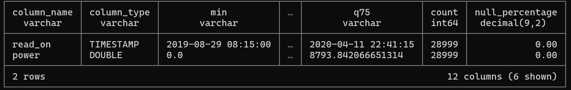
Explanation: The SUMMARIZE keyword automatically generates statistical summaries (mean, min, max, NULL counts, etc.) of result datasets. Useful for quickly understanding data distribution and characteristics during initial data exploration.

Example 7: Subtotal Calculation with GROUP BY ROLLUP

-- Listing 4.13: Hierarchical aggregation using ROLLUP (totals/subtotals)
SELECT 
    year(read_on) AS year, 
    system_id, 
    count(*), 
    round(sum(power) / 4 / 1000, 2) AS kWh 
FROM '/mnt/c/tmp/readings.csv' 
GROUP BY ROLLUP (year, system_id) 
ORDER BY year NULLS FIRST, system_id NULLS FIRST;

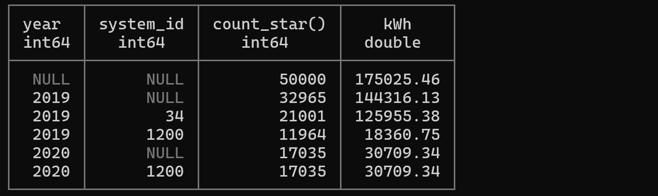
Explanation: ROLLUP calculates hierarchical subtotals. This query generates three levels of aggregation:

1. Aggregation for each (year, system_id) combination
2. Subtotals for each year (system_id is NULL)
3. Grand total (both year and system_id are NULL)

Very useful when hierarchical summaries are needed in reports or dashboards.

Example 8: All Combination Aggregation with GROUP BY CUBE

-- Listing 4.14: Multidimensional aggregation using CUBE
SELECT 
    year(read_on) AS year, 
    system_id, 
    count(*), 
    round(sum(power) / 4 / 1000, 2) AS kWh 
FROM '/mnt/c/tmp/readings.csv' 
GROUP BY CUBE (year, system_id) 
ORDER BY year NULLS FIRST, system_id NULLS FIRST;

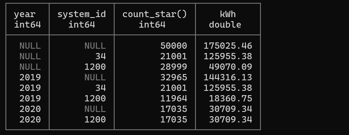
Explanation: CUBE generates aggregations for all possible combinations of specified columns. This query generates four aggregations:

1. (year, system_id) - Each year and system combination
2. (year, NULL) - Total for all systems by year
3. (NULL, system_id) - Total for all years by system
4. (NULL, NULL) - Grand total

Suitable for multidimensional analysis similar to OLAP cubes.

Example 9: Conditional Aggregation Using FILTER

-- Create view
CREATE OR REPLACE VIEW v_power_per_day 
AS SELECT system_id, 
          date_trunc('day', read_on) AS day, 
          round(sum(power) / 4 / 1000, 2) AS kWh, 
   FROM '/mnt/c/tmp/readings.csv' 
   GROUP BY ALL;

-- Listing 4.25: Perform conditional aggregation with FILTER clause (static pivot)
SELECT 
    system_id, 
    sum(kWh) FILTER (WHERE year(day) = 2019) AS 'kWh in 2019', 
    sum(kWh) FILTER (WHERE year(day) = 2020) AS 'kWh in 2020' 
FROM v_power_per_day 
GROUP BY system_id;

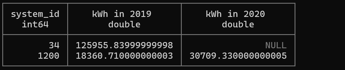
Explanation: The FILTER clause allows applying conditions individually to each aggregate function. This enables performing aggregations with multiple conditions in a single query, making it very efficient performance-wise. Better readability than conditional aggregation using CASE statements.

Example 10: Dynamic Table Transformation with PIVOT

-- Listing 4.26: Dynamic pivot using DuckDB's PIVOT statement
PIVOT (FROM v_power_per_day) 
ON year(day) 
USING sum(kWh);

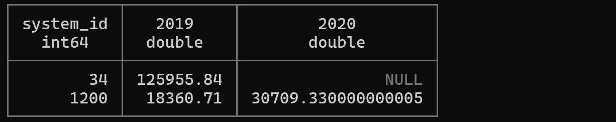
Explanation: PIVOT is a powerful feature that transforms rows into columns. This query creates columns by year and calculates kWh totals for each column. More concise than the previous FILTER approach and dynamically creates columns based on the number of values.

Example 11: Time Series Data Joining with ASOF JOIN

-- Listing 4.28: Time-based approximate join (matching most recent value)
WITH prices AS (
    SELECT range AS valid_at, random()*10 AS price 
    FROM range(
        '2023-01-01 01:00:00'::timestamp, 
        '2023-01-01 02:00:00'::timestamp, 
        INTERVAL '15 minutes'
    )
), sales AS (
    SELECT range AS sold_at, random()*10 AS num 
    FROM range(
        '2023-01-01 01:00:00'::timestamp, 
        '2023-01-01 02:00:00'::timestamp, 
        INTERVAL '5 minutes'
    )
)
SELECT 
    sold_at, 
    valid_at AS 'with_price_at', 
    round(num * price, 2) as price 
FROM sales 
ASOF JOIN prices ON prices.valid_at <= sales.sold_at;

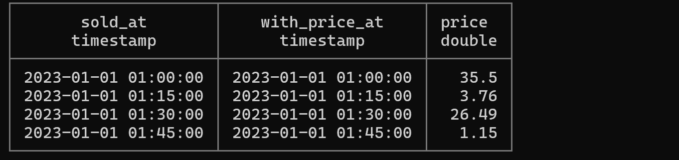
Explanation: ASOF JOIN is a very useful join method for time series data. For each sale time (sold_at), it finds and matches the most recent price (valid_at) before that time. An essential feature when handling time-varying values like financial data and sensor data.

Example 12: CSV to Parquet Conversion and Optimization

# Convert large CSV file to compressed Parquet format
./duckdb -s "
SET memory_limit='1G'; 
COPY (
    SELECT 
        * EXCLUDE (player, wikidata_id) 
        REPLACE (
            cast(strptime(ranking_date::VARCHAR, '%Y%m%d') AS DATE) AS ranking_date,
            cast(strptime(dob, '%Y%m%d') AS DATE) AS dob
        )
    FROM '/mnt/c/tmp/ch05/atp/atp_rankings_*.csv' rankings 
    JOIN (
        FROM '/mnt/c/tmp/ch05/atp/atp_players.csv'
    ) players ON players.player_id = rankings.player
) TO 'atp_rankings.parquet' (
    FORMAT PARQUET, 
    CODEC 'SNAPPY', 
    ROW_GROUP_SIZE 100000
);"

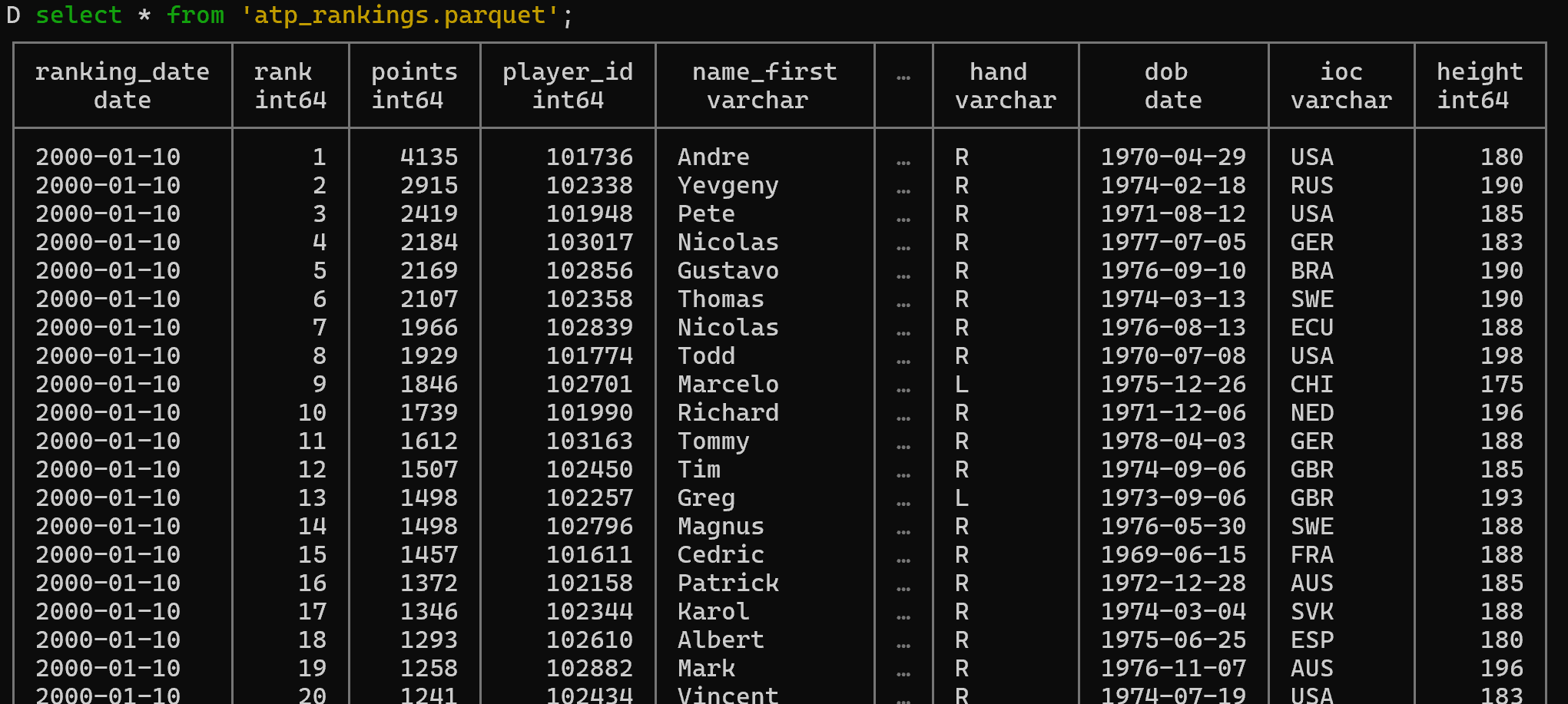
Explanation: This example demonstrates several powerful DuckDB features:

• SET memory_limit: Limit memory usage (OOM prevention)
• EXCLUDE: Exclude specific columns
• REPLACE: Transform column values (string dates to DATE type)
• Read multiple files simultaneously with wildcard pattern (*.csv)
• Export to Parquet format (SNAPPY compression, Row Group size optimization)

This is a practical example of converting CSV to high-performance format in data pipelines.

4. Conclusion

DuckDB's Data Analysis Advantages and Limitations

Key Advantages Summary:

1. Excellent Analytical Performance: Very fast large-scale data analysis with columnar storage and vectorized engine.
2. Zero-ETL Philosophy: Simplifies data pipelines by allowing direct queries on CSV, Parquet, and JSON files.
3. Developer-Friendly: Low learning curve with standard SQL support and intuitive extended syntax.
4. Fully Embedded: Integrates into applications without separate servers or infrastructure.
5. Modern SQL Features: Provides powerful analytical features like PIVOT, ASOF JOIN, and COLUMNS expressions.
6. Scalability: Can process data exceeding memory with disk spilling.
7. Data Science Integration: Seamlessly integrates into data science workflows with perfect Python and R integration.

Limitations to Consider:

1. OLTP Unsuitable: Not suitable for transaction processing or high-frequency write operations.
2. Concurrency Limitations: Only supports single-process writes, limiting multi-user environments.
3. Lack of Network Features: Does not support client-server model by default.
4. Index Limitations: Traditional B-Tree indexes are limited, relies on columnar scans.

Use Cases Where DuckDB Excels:

• Local data analysis and exploration
• Intermediate processing layer for data science projects
• Data transformation in ETL pipelines
• Embedded analytical applications
• Prototyping and development environments
• CSV/Parquet file-based data warehouses

Use Cases Where DuckDB is Not Suitable:

• Online Transaction Processing (OLTP) systems
• Applications requiring multi-user concurrent writes
• Environments requiring client-server architecture
• Real-time high-frequency data ingestion

DuckDB is a tool faithful to its goal of being "SQLite for databases," providing a powerful and easy-to-use solution optimized for analytical workloads. In appropriate use cases, DuckDB delivers exceptional value in both development productivity and query performance.